

Using the Trace Math Function on a CMT Vector Network Analyzer
April 21, 2025By Brian Walker, Sr RF Engineer, SME
The trace math feature of a Copper Mountain Technologies Vector Network Analyzer (VNA) is very useful. This application note will give a few examples of its use.
Getting Started with Trace Math in VNA Software
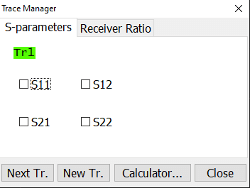
On the VNA UI, click on the S-Parameter callout in the top left corner.
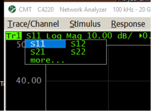
Choose “more…”
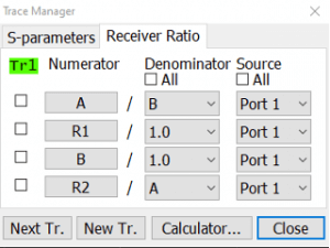
This panel can be used to operate on the trace highlighted in green. If another active trace should be used, click on “Next Tr.” to switch to it. “New Tr.” may be used to add a new trace and switch to it.
Column one lists the four VNA receivers. R1 and R2 are the reference receivers, which monitor the signals leaving ports 1 and 2, respectively. A and B receivers monitor signals entering ports 1 and 2, respectively. Selecting “1” for the denominator and clicking the checkbox will show the signal on that receiver.
Selecting A/R1 with the Port 1 source active allows you to view an uncorrected version of S11. Similarly, selecting B/R1 with the Port 1 source active will enable you to view an uncorrected version of S21. Uncorrected S12 is A/R2, and S22 is B/R2, both with Port 2 active.
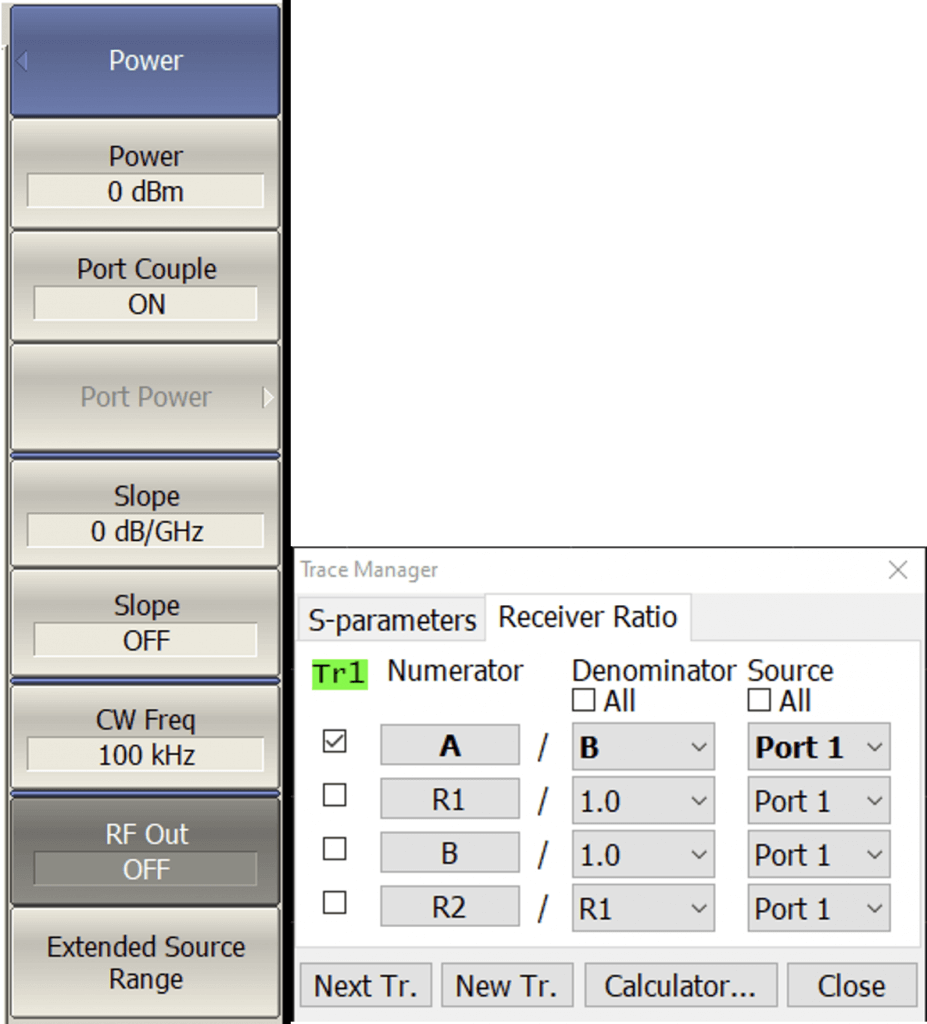
Examining the phase and magnitude relationship between two signals entering ports 1 and 2 is also possible. First, turn off the internal signal source by navigating to Stimulus/Power and clicking on RF Out. Click on “Start” in the lower-left corner of the UI, switch to “Center,” and enter the frequency that will be applied. In the lower-right corner, set the span to 0. Consider setting the IF bandwidth as wide as possible to ensure that the external signal is captured. Choose A/B or B/A on the calculator to see the ratio between the two signals. It doesn’t matter which source port is selected since the power is turned off. The two input signals must be the same frequency, perhaps receiving a signal with two antennas or looking at the phase shift on the two output ports of a 90-degree hybrid.
Choosing the “S-parameters” tab allows users to change to the standard S-parameters S11, S12, S21, or S22.
Basic Functions
Pushing the “Calculator…” button gives access to the trace calculator’s next “Basic” level. In this calculator, traces and S-parameters may be manipulated in useful ways.
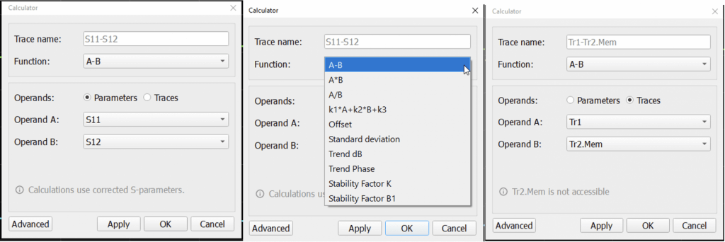
The first few selections perform operations on two linear terms. These terms can be S-parameters, traces, or trace memories. Function A-B subtracts the magnitude of two terms. A*B performs a complex multiplication, A/B complex division. The next function performs a weighted sum of two terms and adds an offset.
The Offset function adds or subtracts a dB value from a term and/or adds a phase offset in degrees. The Standard Deviation function performs a standard deviation function on the linear value of the chosen term. The Trend dB function adds a linear dB slope and an offset to the term. The Trend Phase function performs similarly for the phase of the term in degrees.
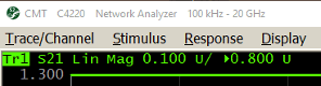
The last two functions are stability factors, which are useful for evaluating an amplifier’s stability. This information is very important for an RF designer. Some off-the-shelf amplifiers are not unconditionally stable and may need additional components to prevent spontaneous oscillation. For example, the MiniCircuits PGA-103+ is an exceptional amplifier with 11 dB of gain, 0.6 to 0.9 dB Noise figure, and a respectable +45 dBm OIP3. The S-parameters can be downloaded from the website and loaded into the VNA. Using the VNA UI, Save/Recall/Load Data from Touchstone File/To S-Parameters, and choose the S-Parameters for the amplifier. Set the trace type to S21 Lin Mag 0.100 U/ 0.800 U.
Open the calculator, select Stability Factor K, and apply. The Rollet stability factor will be displayed. An amplifier is expected to be stable for K values greater than one.
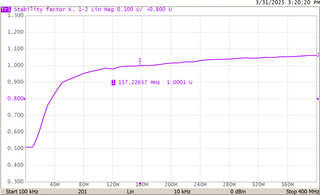
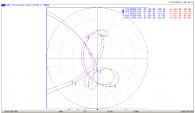
Figure 1 – K Stability Factor
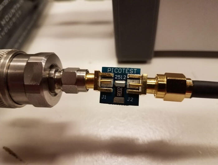
Here, the K stability factor is less than one below 157 MHz in Figure 1, indicating potential instability in that region. The data sheet for the PGA-103+ recommends adding a 620 nH inductor, a 150 ohm resistor and a 330 pF capacitor all in series to ground and attached to the input of the amplifier as shown below.
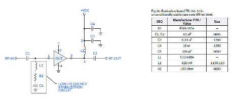
Adding the suggested network results in a K factor greater than 1, as shown in Figure 2 (violet trace), and the amplifier should now be unconditionally stable.
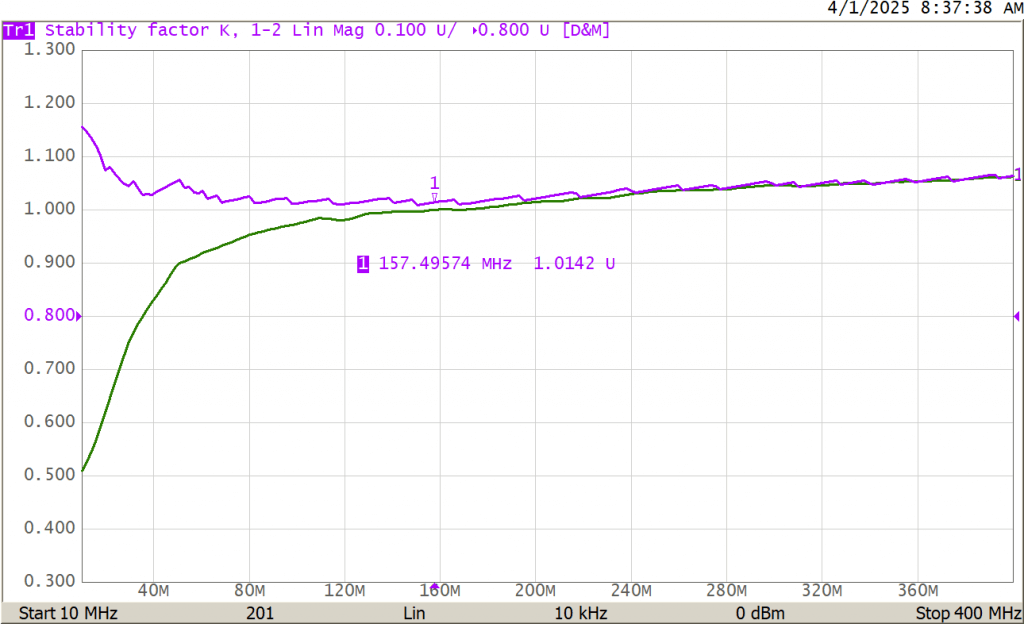
Figure 2 – Stabilized amplifier
As a follow-up, the VNA can measure the amplifier’s performance in its final circuit configuration, and stability may be checked once again in situ. If the measurement is made with soldered-in pigtails, it would be beneficial to de-embed them using the Automatic Fixture Removal program (AFR) from Copper Mountain Technologies.
Finally, for guaranteed stability, it is necessary but not sufficient that the stability factor K be greater than one; An additional stability measure B1 should also be greater than zero. This is the last choice on the calculator menu.
The Advanced Calculator
Pressing the “Advanced” button takes us to the advanced calculator UI.
The “Functions” menu contains a selection of trigonometric, log, and other functions. The “Traces” menu allows for the selection of different kinds of trace data. To make sense of the trace designations, refer to the block diagram of Figure 3.
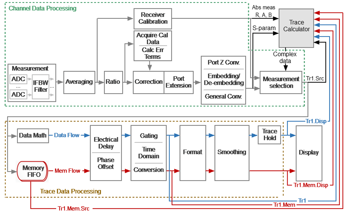
Figure 3 – Data types
For example:
Tr1.Src:
Calibrated complex reflection coefficients, potentially with Port Extension, Port Z conversion, Embedding or De-Embedding, or General Conversion
Tr1:
Tr1.Src with added potential Data Math, Electrical Delay or Phase Offset, Time Domain, Time Domain Gating, and Impedance Conversion, but no Formatting or Smoothing.
Tr1.Mem:
Outputs the memorized Trace 1 data with the same parameters as Tr1
Tr1.Disp:
Tr1 with added Formatting and potential Smoothing applied.
The next column allows for the choice of S-parameters or raw receiver data. The designation R1_1 refers to the Port 1 reference receiver, which monitors the incident output signal with the stimulus switched to exit Port 1. T1_1 refers to the Port 1 reflection receiver, which monitors signals entering Port 1, with the stimulus switched to exit Port 1. R1_2 seems silly since there should be no signal on the Port 1 reference receiver when the stimulus is switched to Port 2, but it is helpful for some special cases involving a Direct Receiver Access VNA.
Differential Calculation
A 2-Port VNA may be used to measure differential return loss by calculating the differential parameters from unbalanced measurements made by each port. That is:
![]()
Enter this into the calculator as (S11+S22-S21-S12)/2. The S-parameters may be chosen from the menu selection, typed into the Expression field by hand, or pasted from a text document. This would allow the user to examine a twisted pair and see the differential return loss. Additionally, the time domain analysis function, a standard feature in most CMT VNAs, may be used to evaluate reflection vs. distance along the twisted pair to detect any breaks or abnormalities.
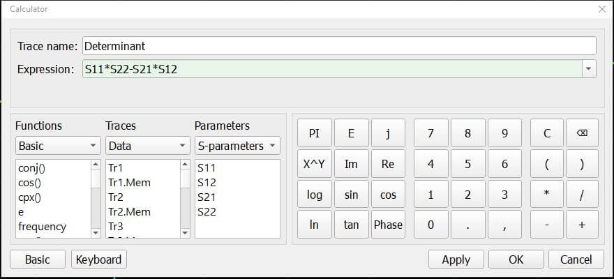
The S-Parameter Determinant
The magnitude of the determinant of the S-parameter matrix S11*S22-S21*S12, tells us something about a 2-port network. If it is equal to one, then the network is lossless. A magnitude greater than one for an amplifier with potential instability. A magnitude less than one typically indicates power loss.
Helpful Hint: It is recommended to keep a text document with a set of favorite functions which can be cut and pasted into the calculator expression field.
Pi-Network Extraction
Consider the Pi network in Figure 4. The three admittances, Y1, Y2, and Y3, can be extracted from the network’s Y-parameters.
The Y-parameters can be found from the S-parameters easily (with Y0 = 1/50).
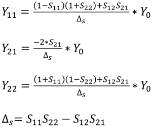
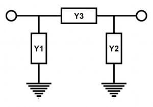
Figure 4 – PI Network
For a Pi-network:
Y1 = Y11 + Y21
Y3 = -Y21
Y2 = Y22 + Y21
In the calculator (for 50 ohm S-parameters):
Y1 = (1/50)*((1-S11)*(1+S22)+S12*S21-2*S21))/(S11*S22-S12*S21)
Y3 = (1/50)*(2*S21)/(S11*S22-S12*S21)
Y2 = (1/50)*((1+S11)*(1-S22)+S12*S21-2*S21))/(S11*S22-S12*S21)
If Y1 were known to be a capacitor, one could plot the value of that capacitor:
C1 = Y1/(2*pi*frequency)
C1 = (1/(2*PI*frequency))*(1/50)*((1-S11)*(1+S22)+S12*S21-2*S21))/(S11*S22-S12*S21)
If Y3 were known to be an inductor, one could extract that value as well:
L3 = -1/(2*PI*frequency*Y3)
L3 = (-1/(2*PI*frequency))*1/((1/50)*(2*S21)/(S11*S22-S12*S21))
It is easy to see how this method could be used to extract lumped element values from measured S-parameters. The location of the reference plane is crucial, however; it must be located right at the component position. Port extension or de-embedding should be employed to ensure this.
Instead of calculating the Y-parameters, one could use General Conversion under the Analysis menu to display Y11, Y21, and Y22 on three traces. Then, the VNA can do that conversion, and the previous calculations can be performed by choosing traces Tr1, Tr2, or Tr3 as needed.
T-Network Extraction
To extract a T-network as in Figure 5, use Z-parameters.
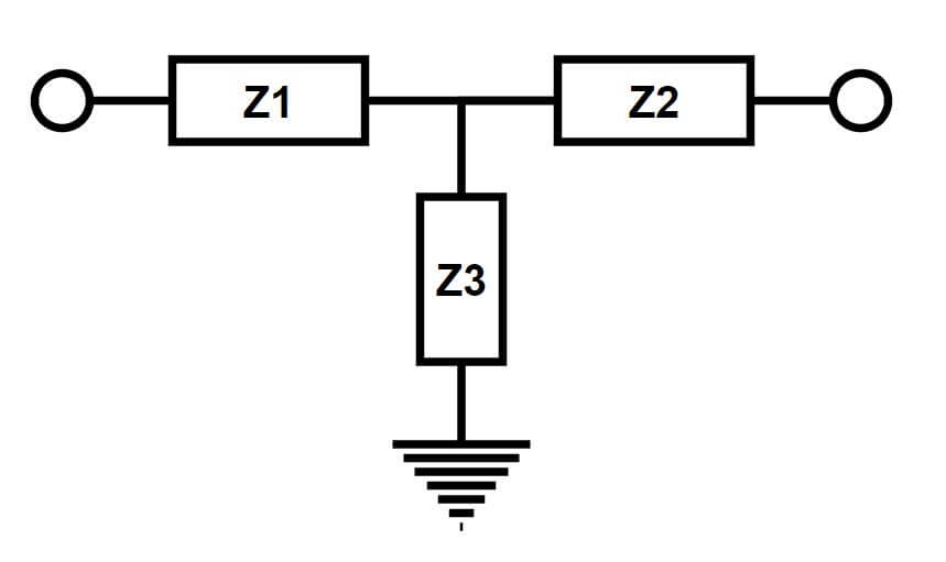
Figure 5 – T-Network
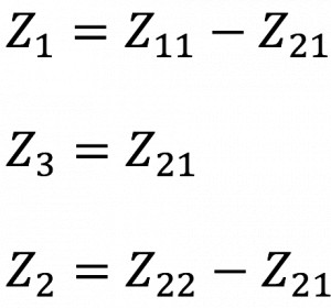
Where:
The Z-parameters may be calculated from S-parameters as follows (with Z0=50):
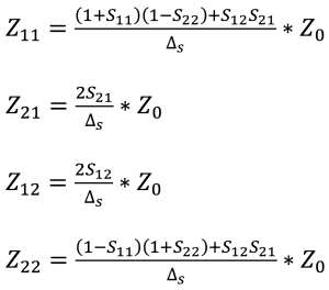
Where
![]()
Then:

Z1 may be entered in the calculator as follows:
50*((1+S11)*(1-S22)+S12*S21-2*S21)/(S11*S22-S12*S21)
And Z2:
50*((1-S11)*(1+S22)+S12*S21-2*S21)/(S11*S22-S12*S21)
And Z3:
50*2*S21/(S11*S22-S12*S21)
These two methods might be used to better understand a device. If the S-parameters of an amplifier are known, the first element of the T-network, Z1, might be the component’s internal bond-wire inductance. An RLC model of an inductor, containing all parasitic values could be created from its S-parameters and used for more accurate simulation. The primary, secondary and mutual inductance of a transformer can be found by modeling it as a Pi-network and finding Y1, Y2 and Y3.
Conclusion
These are just some calculations that might be performed using trace math. We’ve seen how the amplitude and phase of two signals may be compared, how the stability of an amplifier can be verified, how differential measurement conversion is done, and how Pi or T network models might be generated from S-parameters. Many more applications are possible, limited only by the user’s creativity. Trace math is just one of many advanced features available on a Copper Mountain Technologies VNA. Visit our website to see our lineup of equipment and check out our other application notes, videos, and webinars to help you better understand Vector Network Analysis and get more out of your measurements.
Related Post

What is the Difference Between TDR and VNA Time Domain Measurement
September 18, 2023
While both TDR and VNA time domain measurements serve the common purpose of analyzing reflections in RF systems, they differ significantly in methodology, instrumentation, and scope of applications. Learn more in this application note from Brian Walker.
Amplifier Measurements
August 31, 2022
RF amplifiers are an important part of many RF system designs and it is often required to make Vector Network Analyzer (VNA) measurements of them to verify function and ensure suitability for the intended application. Learn about the challenges of different methods for measuring amplifiers with a VNA to achieve accurate, reliable results.
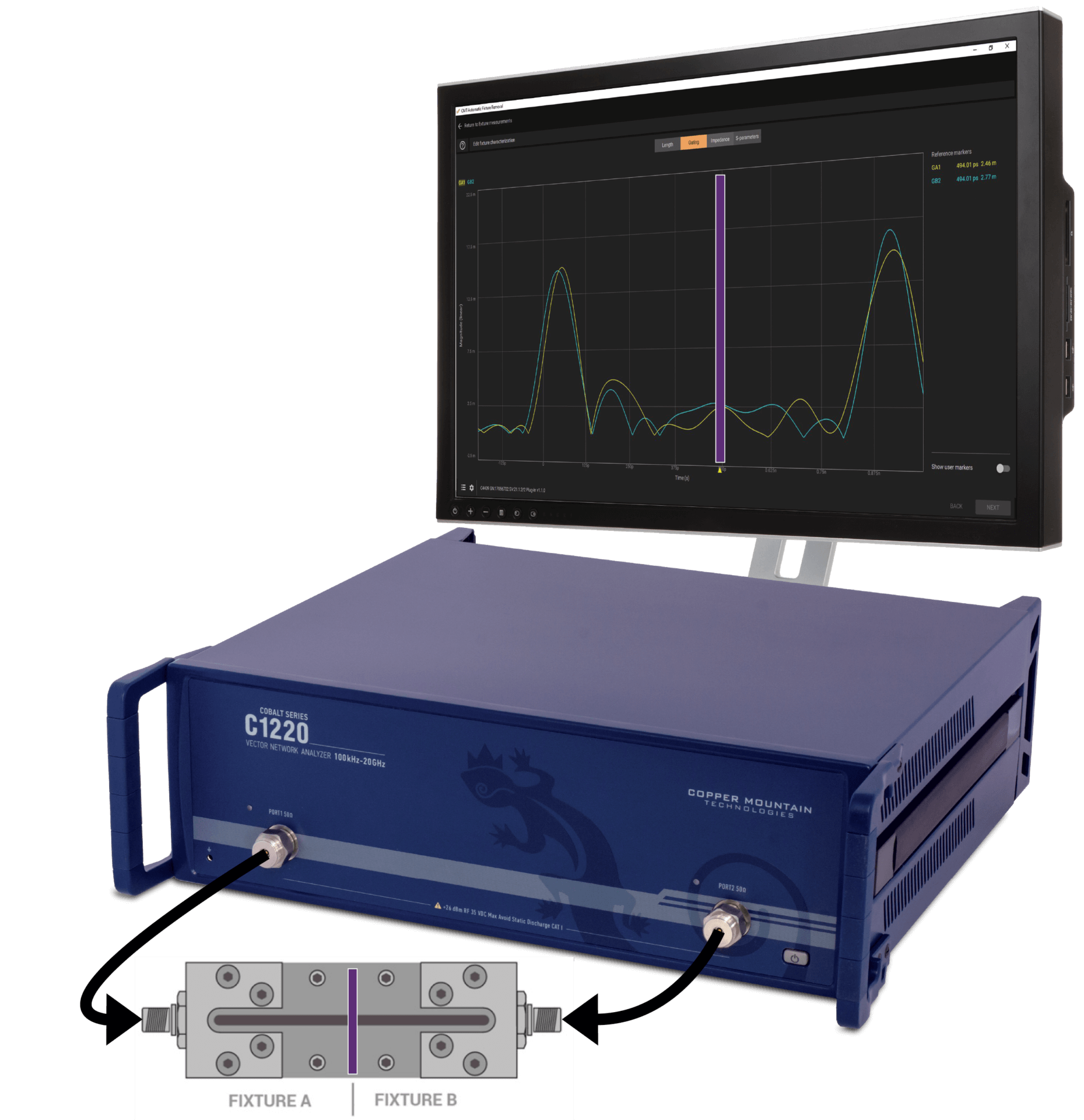
Eliminating Fixture Effects from Embedded Measurements
July 29, 2022
Using the methods in the Automatic Fixture Removal software provides a way to characterize fixtures that could not be done in any other way. A fixture is usually not connectorized at the DUT interface, and attaching a connectorized pigtail is problematic as the pigtail itself would need to be removed from the measurement. The method works best with a wide-band measurement, but the fixture may not support this, so a reduction in the bandwidth may be required to obtain reasonable results. Learn more about this by reading the full application note.
Make Accurate Impedance Measurements Using a VNA
June 21, 2019
Three different methods can be applied to accurately measure passive components with a vector network analyzer. A vector network analyzer (VNA) is a very useful test instrument for characterizing RF circuits and amplifiers. But what about measurements of simple passive components? What’s the best way to characterize a chip capacitor or an inductor—or even a resistor? Senior RF Design Engineer Brian Walker at Copper Mountain Technologies wrote an article for Microwaves & RF discussing how to make accurate impedance measurements using a VNA.
Passive RF System Measurements in a Strong RF Environment: Using an Amplifier with a 2-Port VNA
April 19, 2018
It is sometimes necessary to evaluate passive RF systems in environments where there is significant ingress from other sources. The most common cases are antenna system measurements at community transmitter sites. If there is sufficient RF present in the near field, the antenna being tested doesn’t even need to be particularly broadband for problems to arise. Vector network analyzers are sensitive instruments, typically operated at very low signal levels. Ingress from local sources can skew measurements, and if the ingress is strong enough the analyzer can be damaged. Coordinating multiple station sign-offs can be difficult, if not impossible. When working with broadband antennas in a large market, the interferer doesn’t even need to be collocated to impact the measurements. With another repacking of broadcast spectrum looming, the congestion will only get worse.