To obtain optimal performance in an over the air RF system, the antennas must be chosen to meet specific requirements. Performance parameters such as size, wind-loading, environmental ruggedness, transmission pattern, bandwidth, and power handling capability should be considered. Especially important in an RF system design is the “link budget”. This parameter determines the end-to-end RF loss and is affected by transmitter output power, feedline loss, transmit antenna gain, path loss through the air, receiver antenna gain, feedline loss once again and receiver noise-figure among other factors. A failure to meet the link budget in an RF system design will result in noisy performance and loss of coverage. In this application note, methods of measuring the transmission (or reception) pattern which determines antenna gain with a VNA will be examined.
Radiation Pattern
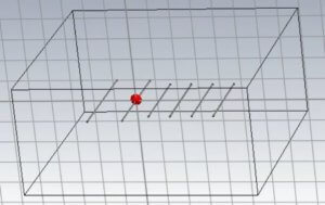
Most antennas possess some directionality to their performance. Even an omnidirectional vertical antenna is usually designed to restrict broadcast to a horizontal plane. Power radiated upwards into space is wasted. A Yagi antenna with a single reflector and multiple directors might look something like what is shown in Figure 1 where the drive point is shown in red.
Figure 1 – Yagi Antenna
The radiation pattern for this structure will be similar to what is shown in Figure 2. Clearly, most of the radiated energy is in a single direction. This result was derived by simulation, but it would be advantageous to measure an actual antenna, one made from real metals instead of perfect conductors and operating in a physical environment with soil beneath it and air above it.
Figure 2 – Yagi Radiation Pattern
The fields around the Antenna Under Test (AUT) may be divided into three regions: the reactive near-field, the radiating near-field and the far-field. The E and H fields in the reactive near-field are not orthogonal and this zone extends from the surface of the AUT out to about λ/2π. The radiating near-field with orthogonal E and H fields extends from about λ/2π to 2D2/λ, where D is the largest dimension of the AUT, and the far field is any distance beyond this.
Far field measurement is straightforward with the AUT illuminated by nearly planar waves generated from some distance away. -Note that reciprocity holds such that measurement of received energy vs antenna orientation is equivalent to mapping its transmission properties- Testing is performed by rotating the AUT Ф around its vertical axis and tilted to different azimuths Θ while the received signal strength is measured.
Figure 3 – Far Field Measurement
In this simple set-up, a CW signal source from a signal generator is broadcast from the far source and Port-2 of the VNA is attached to the AUT with IF Bandwidth set wide enough to account for any small frequency discrepancy between the signal source and the VNA. The VNA will be set to make an absolute measurement of the “B” receiver with the source port arbitrarily set to port 1. A proper understanding of the VNA receivers is needed.
The VNA Receivers
Figure 4 depicts a block diagram of a 2-Port VNA. Each port has two receivers associated with it, one to sample the level of the incident signal leaving the port and the other to measure signals entering it. There is a long legacy of names associated with the receivers and it can be confusing. The receiver which measures the incident signal is called the “Reference” receiver and designated by the letter “R”. It is called the reference receiver because the phases and amplitudes of signals received by this port as a reflection or other ports as transmissions will be referenced to it. The reference receivers are denoted by R1 and R2 or R1 through R4 in the Absolute measurement section of the S2VNA or S4VNA UI software and by “Ref 1”, “Ref 2”, “Ref 3” and so forth on the front panel access ports of a Direct Receiver Access (DRA) VNA.
Figure 4 – 2-Port VNA Block Diagram
The receivers which measure signals entering a port are either denoted by “A” and “B” for Ports 1 and 2 of a 2-Port VNA or T1 through T4 for a 4-Port VNA in the absolute measurement menu of the UI. The “T” stands for “Test” in this case. These receivers are also be called “Measurement” receivers and denoted by “Meas 1”, “Meas 2”, “Meas 3” and so forth on the front panel of a DRA VNA. These receivers have three naming conventions, “A” and “B” for 2-Port VNAs, “T” for 4-Port and higher VNAs, and “Meas” for the front panel connections of a DRA VNA. The VNA User Interface selections for receiver measurements are shown in Figure 5 below and DRA front panel designations are shown in Figure 6.
Figure 5 – UI Receiver Nomenclature
Figure 6 – DRA Front Panel Layout
Making the far-field AUT measurement
We can now use the VNA receivers to make the measurement shown in Figure 3.
The appropriate menu selection is:
Measurement/Absolute/Receiver B-Source Port 1 on a 2-Port VNA or
Measurement/Test Receiver/T2(1) on a 4-Port VNA model.
This enables the input receiver on Port 2 which will have initial absolute accuracy of ±1.5 dB. For better accuracy, perform power and receiver calibration. Ensure that the VNA start and stop frequencies are set for the right measurement range and attach one of the supported USB power meters. You can select a supported power meter from:
System/Misc Setup/Power Meter
Connect the chosen power meter to the end of a test cable attached to Port-1 and select:
Calibration/Power Calibration/Select Port 1 and
Power Sensor Zero Correction wait for it to complete then
Take Cal Sweep
This will calibrate the output power of Port-1 which is needed to further calibrate the receiver input of Port-2. Remove the power meter from the end of the test cable and connect it to Port-2. Then perform Port-2 Receiver calibration. Choose:
Calibration/Receiver Calibration/Select Port 2 then
Calibrate Test Receiver
Now the “B” receiver on Port 2 – Called “Test” receiver on a 4-Port VNA – is calibrated for accurate absolute power measurements.
It is now a good idea to turn off the stimulus power, so it does not interfere with the measurement of external signals. Go to:
Stimulus/Power/RF Out-Off
Now set the VNA to measure:
Measurement/Absolute/Receiver B-Source Port 1 on a 2-port VNA or
Measurement/Test Receiver/T2(1) on a 4-Port VNA
The source port doesn’t actually matter since the RF power is turned off.
Now click on “Start” in the bottom left corner of the display and change it to “Center”. Set the center frequency to that which will be measured, and on the bottom right of the display, set the span to “0”. The displayed line on the screen will be the AUT received power in dBm. The AUT is then rotated and tilted, and measurements recorded. The next frequency is set up on both the VNA and remote source and the AUT measurements are repeated.
If the signal level at the AUT is very small and the IF Bandwidth must be reduced to improve the signal to noise ratio, it may be necessary to use a GPS conditioned, 10 MHz reference on both the generator and the VNA to ensure that frequency inaccuracy doesn’t cause the signal to fall outside the IF bandwidth. The frequencies of the generator and VNA must be coordinated during measurement and this could be done over ethernet or an ISM connection as outlined in this article.
For the measurement configuration of Figure 3 there will be multipath contributions to the line-of-sight signal, particularly one that bounces off the ground. The two signals will constructively or destructively interfere depending on frequency which will put “ripples” in the measurements. A secondary “reference” antenna with flat frequency response may be collocated with the AUT and all measurements ratioed to it to eliminate this error as shown in Figure 7.
Figure 7 – Using a Reference Antenna
The desired measurement is receiver B, (T2 on a 4-Port VNA), divided by receiver A (or T1) B/A. It is possible to measure the absolute A and B receivers and divide the results, but the two receivers are not phase matched to each other and erroneous offsets will be seen. It is much better to measure S21 and S11 with the VNA RF stimulus turned off and then divide the two results. This works because:
then
The S-Parameters are factory calibrated to the output connectors of the VNA, so this ratio gives good, consistent results. The only drawback to this is that R1 is a measurement of the stimulus signal which has been shut off. There is some leakage of the port 1 input signal through the input bridge to the R1 receiver though, enough to make the measurement work but there will be some additional noise when measuring low-level signals. For better performance, one can use a VNA with Direct Receiver Access (DRA) option, a Copper Mountain Technologies C2209, C2409, C2220 or C2420. The signal from the reference antenna is split and applied to both the A receiver (Meas 1) and the R1 receiver (Ref 1). This gives a cleaner measurement since R1 is properly defined.
Figure 8 – Measurement with DRA
For mmWave measurement, the far-field might be as short a distance as 77 cm. For this case, the measurement could be conveniently performed with a small anechoic chamber such as those offered by Millibox. The chamber in Figure 9 might be used for characterizing antennas in the 18 to 95 GHz range.
Figure 9 – Millibox MBX02 Test Chamber
The RF absorbers in the chamber reduce reflections from the walls by 50 dB at normal incidence. To better this, one would apply time domain gating to accept only signals originating from the AUT and reflections from the chamber sides and back would be rejected. Time domain gating is an advanced feature common to all Copper Mountain Technologies VNAs except for the “M” series models. See our application note and video on this feature for more information.
Microwave Vision Group, MVG, also provides hardware and software for near and far-field antenna measurement. VNAs from Copper Mountain Technologies are integrated into their test and analysis software.
A Gating Example
A microwave horn was attached directly to an R180, 18 GHz 1-Port VNA. A metal object was placed in front of the horn as shown in Figure 10. Behind the metal target are other reflecting objects.
*The R180 has been discontinued. R140B is a suitable option for most 1-Port use cases.
Figure 10 – 1-Port VNA with horn
In the Time Domain mode, the target is clearly seen along with background “clutter”.
Figure 11 – Time Domain Reflections
By applying “bandpass” gating, the reflection from the target can be singled out and all interfering reflections eliminated.
Figure 12 – Gated Target
Gating like this would be appropriate for antenna measurement to eliminate reflections from walls and other objects.
Near-Field Measurement
It is often much easier to evaluate an antenna using near-field measurement. The infrastructure needed to make the measurement is smaller and less expensive and environmental factors such as wind and rain are not an issue. Actual measurements consist of a mixture of radiating and non-radiating near-field and far-field electromagnetic energy. To accomplish this, a probe which measures the electric or magnetic field is moved within a plane in a grid with intervals of less than λ/2. The plane should be large enough to encompass a majority of the emitted energy. Essentially, each measured point may be considered to be a point source radiator and the far-field pattern may be calculated from the contribution of each. This calculation is identical to a two-dimensional discrete Fourier transform of the measured data points.
Figure 13- Near Field Measurement
The measurement may also be performed with a sampled spherical or cylindrical surface. Additionally, it is possible to use a Fourier transform to project back to the antenna and determine surface currents on its structure or even determine the shape of an object scattering RF energy. This latter imaging process is called RF holography. High frequencies and small wavelengths give improved resolution for this, but accurate half-wavelength positioning of the measurement probe becomes more difficult. The Insight software from MVG is capable of this sort of analysis.
Antenna Gain Measurement
The gain of an antenna can be measured by comparing its performance to a reference antenna with known gain. Measure S21 of the reference antenna with a generic receiving antenna and normalize the result.
Figure 14 – Gain Measurement
In the VNA UI Menu:
Display/Memory/Normalize
Replace the reference antenna with the AUT and measure S21 once again. This result is the gain difference between the known antenna and the AUT. The data may be saved to a CSV file by selecting:
Save-Recall/Save Trace Data
With known reference antenna data, this difference information can be used to calculate the actual gain of the AUT in a spreadsheet.
Automation
Every CMT VNA can be operated under programmatic control using platforms such as C++, C#, Python, VBA, Matlab or LabView. In the VNA User Interface, a port can be enabled and SCPI commands can be issued to the VNA to effect measurements and receive data. This is important because program automation would normally be used to position an AUT and then to perform and record measurement results. Example code can be found online here and a helpful automation guide is here. The latest VNA UI software, S2VNA, S4VNA and RVNA is available on the website and may be downloaded and run in “demo” mode for testing automation software. There is a great two minute introduction to VNA automation here and a more detailed “bootcamp” video here.
Conclusion
A VNA is an important tool for antenna characterization. Compact VNAs from Copper Mountain Technologies are ideal for making these measurements in the field. The Cobalt series VNAs with their high dynamic range are a great choice for use in the lab. All CMT VNAs are integrated with turnkey measurement solutions offered by MVG and Millibox. For more information about CMT products, please visit our website at www.coppermountaintech.com. For detailed application information feel free to contact our technical support team at support@coppermountaintech.com or call 317-222-5400 and ask for Applications Engineering.
To provide the best experiences, we use technologies like cookies to store and/or access device information. Consenting to these technologies will allow us to process data such as browsing behavior or unique IDs on this site. Not consenting or withdrawing consent, may adversely affect certain features and functions. We will not sell your information to third parties.
Functional
Always active
The technical storage or access is strictly necessary for the legitimate purpose of enabling the use of a specific service explicitly requested by the subscriber or user, or for the sole purpose of carrying out the transmission of a communication over an electronic communications network.
Preferences
The technical storage or access is necessary for the legitimate purpose of storing preferences that are not requested by the subscriber or user.
Statistics
The technical storage or access that is used exclusively for statistical purposes.The technical storage or access that is used exclusively for anonymous statistical purposes. Without a subpoena, voluntary compliance on the part of your Internet Service Provider, or additional records from a third party, information stored or retrieved for this purpose alone cannot usually be used to identify you.
Marketing
The technical storage or access is required to create user profiles to send advertising, or to track the user on a website or across several websites for similar marketing purposes.
To provide the best experiences, we use technologies like cookies to store and/or access device information. Consenting to these technologies will allow us to process data such as browsing behavior or unique IDs on this site. Not consenting or withdrawing consent, may adversely affect certain features and functions.
Functional
Always active
The technical storage or access is strictly necessary for the legitimate purpose of enabling the use of a specific service explicitly requested by the subscriber or user, or for the sole purpose of carrying out the transmission of a communication over an electronic communications network.
Preferences
The technical storage or access is necessary for the legitimate purpose of storing preferences that are not requested by the subscriber or user.
Statistics
The technical storage or access that is used exclusively for statistical purposes.The technical storage or access that is used exclusively for anonymous statistical purposes. Without a subpoena, voluntary compliance on the part of your Internet Service Provider, or additional records from a third party, information stored or retrieved for this purpose alone cannot usually be used to identify you.
Marketing
The technical storage or access is required to create user profiles to send advertising, or to track the user on a website or across several websites for similar marketing purposes.