What is a Waveguide?

A waveguide is rectangular, circular, or oval “pipe” filled with air or dielectric material which is capable of conveying RF energy. The physical implementation of the structure determines the frequencies which may be transported. Many Eigenmodes are possible, but the lowest order is almost always used. Equations for the calculation of these modes for rectangular waveguides are detailed below. A chart of common commercially available waveguides is also included at the page’s conclusion.

What are the Transverse Electric (TE) and Transverse Magnetic (TM) Modes?

An example of waveguide structure is shown below in Figure 1:

Figure 1 – Waveguide Structure This structure will support both transverse electric (TE) and transverse magnetic (TM) field modes of propagation. An electromagnetic wave propagating in free space exhibits both conditions – transverse electric and magnetic fields, or TEM mode. For free space propagation, the E and H fields are at right angles to each other, and at right angles to the direction of propagation. The Poynting vector, E X H, points in the direction of signal propagation. This is not the case for signals in a waveguide. Either the electric field is fully in the XY plane with no Z component, or it is in the magnetic field, but never both.

What is Waveguide Cutoff?

The lowest frequency that a waveguide can support is called the cutoff frequency and is always the transverse electric mode of the lowest order, TE₁₀, also called the fundamental mode of the waveguide. The waveguide should be used between its cutoff frequency and the beginning of the range for the next higher order mode, TE₁₁. It is not recommended to operate the waveguide at a frequency where more than one TE mode is supported, since the different modes travel at different speeds and would interfere with each other. 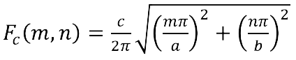The cutoff frequency for each TE_mn mode is given by:

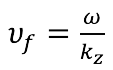
Note that for the fundamental TE₁₀ mode, the b dimension isn’t relevant, and the cutoff equation simplifies to c/2a. The variable b is usually a/2. The equation for the cutoff of a waveguide propagating TM mode waves is the same as the TE equation, except that neither m nor n can be zero. The lowest cutoff is therefore in the TM₁₁ mode. Waveguides are a dispersive media, meaning that the delay vs frequency is not at all flat. The equations of the phase speed and the group velocity are given below. 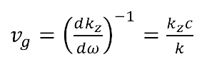The z component of the wave vector, k_z, is given by: