Introduction

A Vector Network Analyzer (VNA) must be calibrated to perform precision measurements. The process of calibration requires the measurement of known calibration standards. A mathematical algorithm takes in the known data of the standards and their measurements to create a correction formula. Systematic measurement errors of the VNA plus test cables and connectors are thereby reduced to very small values, which are called residual errors. Re-measurements of the standards used for calibration will then match the known characteristics, and measurements of unknown devices will be accurate. This is well known to those who study calibration theory.

There are several calibration methods. Among them Short-Open-Load-Thru (SOLT), Short-Open-Load-Reciprocal (SOLR), Thru-Reflect-Line (TRL), and Line-Reflect-Match (LRM).

What are the SOLT Calibration Standards?

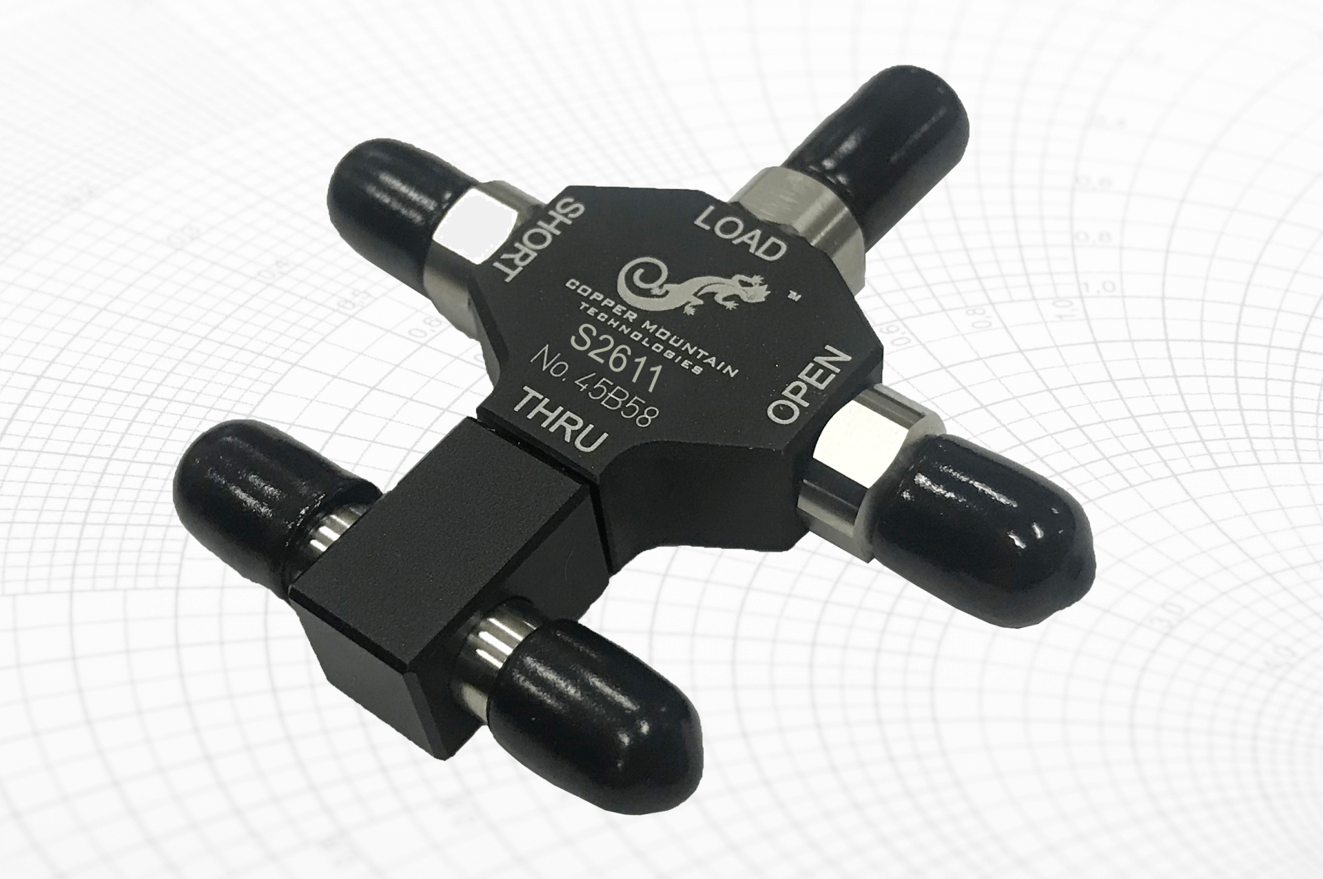
For SOLT, there are Short, Open, Load, and Thru standards. All four of these must be characterized in some way to allow the VNA to know the true measurements of each piece. A mechanical calibration kit, such as the one below in Figure 1 below, is characterized with delay and parasitic data.

Figure 1 – S2611 Mechanical Calibration Kit

The Open is modeled as a delay from the connector to a small parasitic capacitor. The Short is modeled as a delay from the connector to a small parasitic inductor.

The Thru is modeled as a simple delay and the Load is assumed to be perfect. This is shown in Figure 2.

Figure 2 – S2611 Cal Kit Model

The parasitic capacitance and inductance are characterized by a third order polynomial with frequency.

These values are entered in the VNA calibration kit definition so it can calculate the true reflection data for each piece.

Figure 3 – S2611 Cal Kit Definition in VNA Software

For better accuracy, each of the calibration standards might be measured by what is called a golden VNA; calibrated with very expensive primary standards and with the results saved to Touchstone files. These files may then be used to create a data-based definition for each of the standards. This approach is much more accurate than the polynomial approximation, but is quite expensive, as the characterization must be performed on each standard on an individual basis. The calibration kit definition for a set of data-based standards looks like what is shown in Figure 4. The three one-port Touchstone files for Open, Short, and Load, and the one two-port file for the Thru are saved in a separate entry screen.

Figure 4 – Data Based Standards

For those who are familiar with the Smith Chart, you would likely expect the Open standard to be a dot at 0 degrees, and the Short to be a dot at 180 degrees. This is not the case, except for very low frequencies. The delay between the connector and the Short or Open results in a clockwise arc of reflection coefficients as frequency increases. After calibration, and if measured over a wide frequency range, re-installing the Short or Open should produce this arc. The two standards should appear as in Figure 5 and Figure 6, and should not be a dot.

Figure 5 – Typical Open Standard Response

Figure 6 – Typical Short Standard Response

If the Short or Open standard is reattached to a port after calibration is completed, the result must look like what is shown in Figure 5 and Figure 6. For polynomial based calibration, the Load standard will look like a dot in the center of the Smith Chart, since it is assumed to be perfect.

What is SOLR?

SOLR uses the same calibration standards as SOLT, but the Thru need not be characterized. A Thru with unknown characteristics may be used instead as long as its S₁₂ is equal to its S₂₁ (reciprocal response). The delay of the Thru does not need to be known (within reason) and it can be somewhat lossy. Instead of specifying a Thru in the calibration kit definition, choose Unknown Thru as in Figure 3. As an example of how forgiving this method is, it is entirely possible, although not recommended, to use a 10 dB pad as the Unknown Thru for calibration.

The mathematics of the calibration are slightly different between SOLT and SOLR, but the accuracy results are similar. In fact, it is more desirable to choose Unknown Thru, even if the Thru is known. That way, if the Thru standard is somewhat degraded or the connectors aren’t perfectly clean, it won’t matter.

What is a Sliding Load?

The uncertainty (worst case return loss) of the calibration Load is the weakest link in the SOLT/SOLR calibration method. It is not possible to make accurate reflection measurements lower than the Load uncertainty. Data-basing the Load is a huge improvement, but a Sliding Load is nearly as good. If a Load cannot be a perfect 50 ohms but is slightly offset from the center of the Smith chart, it can be put on the end of a precision 50Ω adjustable length air-line. Lengthening the line will cause the measurement to circle around the characteristic impedance of the line, 50Ω –the center of the Smith Chart. If several measurements are made, the center of the circle is easily calculated. This center is a more accurate 50 ohms, as accurate as the characteristic impedance of the air-line, which can be very precise with good machining.

The SOLT method with sliding load simply asks the user to slide the air-line between specified points to allow enough measurements to calculate the center. This measurement replaces the normal Load standard measurement.

What Standards are Used for TRL?

TRL—or Thru, Reflect, and Line calibration— uses two transmission lines and a reflection, such as a Short or Open. The Thru can have zero length, as in the case where the test cables have connectors which mate directly, or it can be a short length of transmission line. The Line must be 20 to 160° longer than the Thru, or 90° longer at the center of the usable band. The Reflect can be a Short or an Open, or any total or near-total reflection. The phase of the reflection at each frequency must be known to the VNA within ±180°, so it is best to specify the internal delay of the reflection.

The Line must also have pristine characteristic impedance with very low reflection. The return loss of the Line sets the bottom limit accuracy for one-port reflection measurements. It is common to use a very expensive air line for this purpose.

Figure 7 – Maury Microwave Airline with Unsupported Center Conductor

Many commercially available air lines have an unsupported center conductor, as in Figure 7, which is held in place only by the end connectors. These Lines are fragile and expensive. The characteristic impedance, however, is precisely known due to the precision machining of the coaxial components. The return loss can be better than 48 dB to 50 GHz. Other Lines have the center conductor supported by internal struts, which makes them more durable but degrades return loss performance somewhat.

The Reflect standard might simply be the Short from a calibration kit, or an end-launch connector which is immediately shorted on the PCB. The performance of the Short is not critical.

TRL does not use a 50Ω load standard, which is usually the weakest link in any calibration kit. A very expensive load standard might have 40 dB return loss, which sets the floor for reflection measurement accuracy, where a precision Line might provide 50 to 60 dB over a narrow frequency band resulting in 10 to 20 dB improvement in the reflection accuracy range.

While it is difficult to support very low frequencies due to the line length requirement, the upper range may be extended almost indefinitely by adding additional Lines with overlapping 20 to 160° lengths to go to higher frequencies. This is called Multi-Line TRL. In other words, at the frequency where the first Line is 155° long, use a second line which is only 20° long at this same frequency. Any number of Lines may be cascaded in this way.

What is an Automatic Calibration Module (ACM)?

An Automatic Calibration Module (ACM) is a device which contains all needed calibration standards that are automatically switched into position during calibration, as shown in the block diagram of Figure 8.

Figure 8 – ACM Block Diagram

The ACM also contains the temperature-corrected data-based data for all SOLT standards, which are uploaded to the VNA prior to performing automatic calibration. The result is a broadband calibration with the best precision possible.  

How is Waveguide Calibrated?

Because waveguide is already band-limited by nature, it is best to use TRL. The Thru is accomplished by attaching the Port 1 and Port 2 waveguide ports directly together for a zero-length Thru. The Line is a 90° length of waveguide at the center frequency of interest and the reflect is a shorting plate placed over each waveguide port in turn. If the Line requirement is too short, use a length which is N*360° + 90°, but this will result in a reduction of the usable bandwidth of the Line.

Alternatively, you may use SOLT or SOLR, but an expensive broadband waveguide Load is required. The Short will be a plate covering the waveguide output, and the Open will be affected by adding a 90° shim in front of the Short to create a 180° phase shift. Leaving the waveguide open is not an effective Open for calibration, since there will be significant radiation from the waveguide aperture.

Conclusion

The major methods of calibration were discussed here. All methods present a number of standards with known characteristics to be measured by the VNA such that errors may be calculated and removed from subsequent measurements. Other methods exist which have not been mentioned, but in general, most methods utilize three or four standards with reflection coefficients with large vector differences. Open, Short, and Load are relatively far apart on the Smith Chart, as would be three reflections which are 120° apart on the circumference.

Achieving the best calibration requires very accurate knowledge of the actual reflection coefficients such that measurements of them allow for optimal calculation of error correction.