Introduction

The examples in this document are based on working with the SC5090 Compact VNA but apply to most of the Copper Mountain Technologies’ VNAs. These tips will help you use your VNA with ease and get more intuitive results.

1. Time Domain Transformation

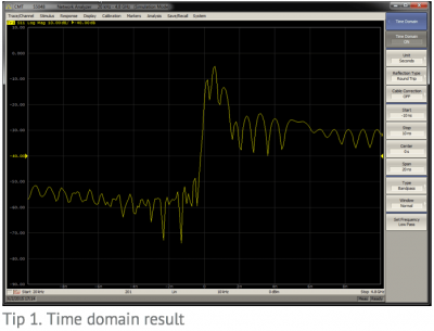
Using Time Domain Transformation will translate the frequency domain result into the time domain by applying an Inverse Fourier Transformation. Time domain measurement can show the length of the transmission line, variations in impedance over distance, responses of individual filters, etc. It can simplify a lot of analysis, such as identifying discontinuities in a transmission line and tuning a particular filter within coupled-resonator filters.

To use this function, choose the active trace and select Analysis -> Time Domain -> Time Domain to transform the trace. The horizontal axis will become nanoseconds and the data is now presented in time domain.

2. Using the Gating Function

Using the gating function can remove the unwanted portion of time domain data and transform it back into frequency domain. It can help remove the effects of a transmission line, connector, etc. as long as its delay is known. It’s one of the simplest ways to de-embed a mismatch and optimize the results when other calibration is not available.

To use this function, you just choose the active trace and select Analysis -> Gating -> Gating to turn on the function. Input the desired start and stop times to acquire the corresponding S-parameter. You can view the plot in the time domain to help with choosing the desired range as well.

3. Using an Automatic Calibration Module

Using the Automatic Calibration Module (ACM), a fast and accurate calibration can be obtained easily. Just connect the ACM to the VNA and set the frequency range of the VNA to be within the limits of the ACM. Then connect the ACM to your computer with the provided USB cable.

To start the calibration process, just choose Calibration -> AutoCal -> 2-Port AutoCal (or 1-Port AutoCal). A highly accurate calibration will be completed automatically.

Under the “AutoCal” menu, you can push the “Confidence Check” button to verify the accuracy of your calibration. This will switch in an internal 20 dB attenuator which has been characterized in the factory. The factory measurement will be loaded into memory and you can compare your measurement to it. The traces should lay on top of each other. Turning on “Data/Mem” math will show you the actual difference which should be within a tenth of a dB or so. Greater differences indicate a problem with cables or connections.

4. Maximizing a Trace

Managing many simultaneous traces can be a challenge. If there are multiple traces in the same window, you can select the active trace at the top of the display and double click on an empty space of the plot. The active trace will be maximized, and all other traces will be hidden. Double click again to toggle between all traces and only the selected trace.

5. Rescaling with the Mouse Cursor

The plot scale and offset can be easily changed without going into the menus.  For the horizontal axis, click and drag the middle number to change the center frequency displayed on the screen. Click and drag any other number to change the span. Click and drag either end, and you will change the start or stop frequency.

For the vertical axis, click and drag any number on the axis to change the offset of the axis. Click and drag either end of the axis, and you change the span of the axis.

6. Saving Results with Print Function

Saving and sharing test results is easy using the print function. Several different options for outputting the picture can be found.

Click on System -> Print, and three different options will appear. MS Word will output a picture into a Word document automatically. Windows will save a PNG file to your computer and open it automatically. Embedded will pop up a print window for the current result automatically.

7. Automation of the VNA

Automatic control of the VNA is straightforward. The VNA can be automated by a set of SCPI-like commands; any language that supports Microsoft COM (aka ActiveX) will be able to communicate with the VNA. Programming examples for MATLAB, C++, C#, Python, VEE, LabVIEW, etc. are provided in the software. Additional guides and examples are available upon request.

8. Updating Settings Using the Mouse

Many of the stimulus and display settings can be changed directly on the plot. Click the parameter in the display, and you will be able to directly change most of them, including span, offset, start and stop frequency, number of points, IF bandwidth, display format, and output power.

Of course, these can also be updated via the menu tree, but often accessing them directly is more convenient.

9. Parameter Conversion

Easy parameter conversion is available. You will be able to view the result as impedance, admittance, inverse- S parameters, and more. In some applications, this can provide a more intuitive representation for the measurement result.

To convert data, click Analysis -> Conversion or Analysis  -> General Conversion to view different formats available.  Click again on Conversion or General Conversion to enable the function.

10. Maximizing Dynamic Range

To maximize the dynamic range of the measurement, you can increase the output power and decrease the IF bandwidth.

When increasing the output power, be careful not to exceed the maximum input range of the device under test, especially amplifiers. Decreasing the IF bandwidth will require a longer time to generate each update of the test result.  However, both of these actions will lower the noise floor of the S-parameter and provide a more accurate result.

References:

S2 Operating Manual – Online Version

S2 Operating Manual – PDF Version

S2 Programming Manual