

Automatic Fixture Removal Operating Manual
July 8, 2021Introduction
Automatic Fixture Removal’s new SW release addresses de-embedding with comprehensive methods, tailored to specific fixture properties. It moves the calibration plane toward hard-to-access components and guides the de-embedding process. Thru, reflect and up to four-port single-ended fixtures are supported. AFR SW supports all CMT two-or four-port instruments.
It guides through the step-by-step process, providing clear instructions and explanations of the step. Description, Fixture Connection, VNA Setup, VNA Calibration, Fixture Measurement, and Result sections show the progression of the de-embedding procedure. Each step includes detailed instructions.
The plug-in executes two-tier calibration – port calibration at the fixture connection plane and fixture calibration at the DUT connection plane. Fixture parameters are then de-embedded.
Errors and Warnings provide clear indicators of possible issues. They are displayed at various places on the screen and are easily understood. The notification area collects all messages and shows them in chronological order.
Setup area indicates Settings, License, and Display information.
Description

Figure 1: Description
Description denotes initial fixture settings, such as ports on each side of the fixture, de-embedding methods, recalls previous settings if available. It is also possible to return the plug-in to the preset mode from this screen.

Figure 2: Initial Fixture Settings
Number of ports cannot exceed the number of available VNA ports.
AFR Plug-in supports 2xThrough and Reflect fixtures. SE indicates Single Ended fixture connection.

Figure 3: De-embedding Methods
There are three methods that fit different fixture configurations:
- Time-gating approach works for fixtures with long electrical length of leading transmission lines or for higher frequency options.
- Filtering algorithm is used in cases where signals in both parts of the fixture significantly overlap in time domain.
- Bisect method covers instances with short electrical length of the fixture leading transmission lines and inadequate time domain resolution.

![]()
Figure 4: Instructions Icon
Pressing the question mark icon opens instructions. Each step has this button. Instructions can be undocked from the main application window. Instructions for all steps are provided in Appendix.
![]()
Figure 5: Notifications Icon
All notifications are collected in Notification Field accessible by pressing Notification Icon. Pressing the icon second time closes the field.
![]()
Figure 6: Setup Icon
Setup Icon gives access to Settings, License information, and Display Scale.

Figure 7: Settings: Monitor theme, User Setup Save, Network IP, and Port

Figure 8: Settings: License Information

Figure 9: Settings: Display
Fixture Connection

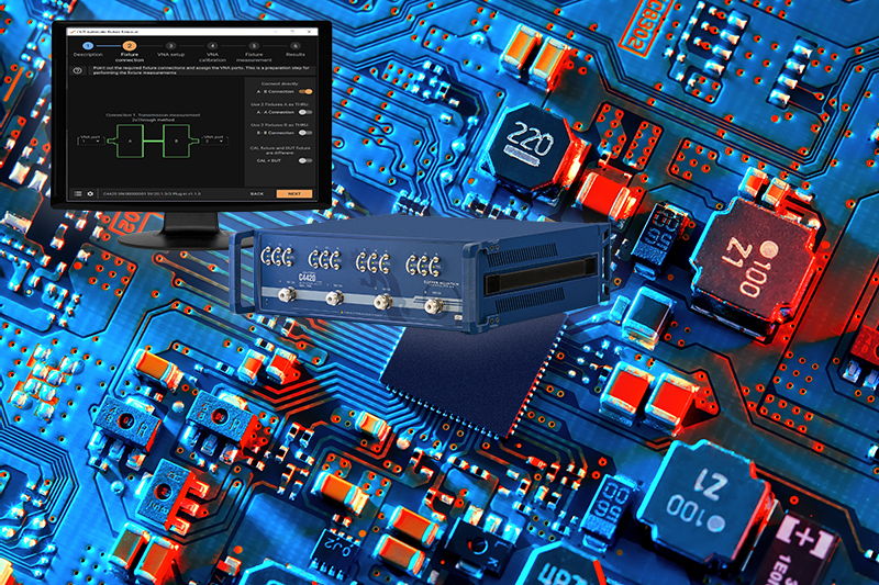
Figure 10: Fixture Connection: 2xThrough Fixture Configuration
Fixture Connection step defines connections to the VNA and Fixture Configuration. Fixture Configuration is flexible and supports 2xThrough and 1xReflect variations, as well as identical fixtures. Instructions under ![]()

Figure 11: Fixture Connection: 1xReflect Fixture Configuration

Figure 12: Fixture Connection: Identical halves – 2xThrough
VNA Setup

Figure 13: VNA Setup: Recommended Settings
VNA Setup step guides the user through VNA settings, including Low Pass mode and Impedance. It shows recommended stimulus parameters and compares them to the current values. Instructions under ![]()

Figure 14: VNA Setup: Warning example
If VNA settings do not follow recommended values a Warning will appear and give further context to explain the issue.
VNA Calibration

Figure 15: VNA Calibration
VNA calibration step displays recommended calibration mode. It must be performed by the user through VNA GUI. The plug-in shows critical errors preventing further steps if calibration is not performed. Instructions under ![]()

Figure 16: VNA Calibration: Critical Error example

Figure 17: VNA Calibration: After calibration is performed
Fixture Measurement

Figure 18: Fixture Measurement
Measure button starts fixture characterization. It is possible to recall fixture parameters and delete data. Instructions under ![]()

Figure 19: Edit Fixture Characterization
Edit characterization graphs
- Length displays the impulse response of the circuit from which the electrical length is estimated. To calculate this, the 2xThrough transmission coefficient data or 1xReflect reflection coefficient data is used.
- Gating displays the impulse response of the circuit with an indication of the time gating range. The calculation uses the 2xThrough reflection coefficient and the 1xReflect reflection coefficient with maximum signal suppression. The characteristic can be used to judge the quality of the fixture, i.e. the presence of heterogeneities in its design.
- Impedance displays the fixture impedance along its length. The characteristic shows how much the impedance changes and what its value is in the connection area of the DUT. A deviation of impedance from the required value by more than 5-10% can further lead to significant distortions in the measurement results of the DUT.
S-parameters display the calculated parameters of each fixture in the frequency domain.
Results

Figure 20: Results
Results step contains Apply, Save Correction Files, Save Setup, and Save Raw Data options. Instructions under ![]()
Appendix
AFR Plug-in Instructions
Step 1. Description
The Fixture description tab allows for selection of the configuration of the fixture with a DUT, as well as the correction method of calculating the fixture parameters.
While on this tab, the following would have to be confirmed:
- The selected configuration Fixture A – DUT – Fixture B corresponds to the actual DUT configuration;
- The analyzer has enough ports for connection.
Note:
The fixture is the device to which the DUT will be connected at the time of measurement.
It is assumed that the user does have a calibration kit to calibrate the analyzer in the connection plane of the DUT.
Procedure:
- Check that the number of analyzer ports is sufficient to connect the DUT in the fixture.
Also, make sure that the types of analyzer test port connectors match the fixture connectors.
- Select the required number of Fixture A port(s) from the list. If Fixture A will not be used, it can be disabled.
- Select the required number of Fixture B port(s) from the list. If Fixture B will not be used, it can be disabled.
- Select the appropriate method for calculating fixture parameters from the list.
The plug-in uses metrology grade de-embedding algorithms to eliminate fixture effects on a DUT. CMT offers 2xThrough (transmission measurement) and 1xReflect (reflection measurement) fixture removal support with three methods that fit different fixture configurations:
- Time gating is ideal for fixtures having leading transmission lines with long electrical length or for higher frequency options. It supports both 2xThrough and 1xReflect.
This method should be used when the electrical fixture length is greater than 4x the rise time. It is acceptable to have some impedance variations along the fixture length.
- Filtering is the most accurate method in cases where signals passing through the fixture significantly overlap in time domain and are difficult to separate from each other. It supports both 2xThrough and 1xReflect.
This method should be used when the electrical fixture length is greater than or close to 4x the rise time and there are no impedance variations along the fixture length.
- Bisection method can be used when the fixture has leading transmission lines with short electrical length and inadequate time domain resolution. This is the most basic method. It does not perform processing in time domain. Bisection method supports 2xThrough only.
This version of the plug-in works only with Single Ended (non-differential) ports. This is shown in the figure as SE.
If the selected number of Fixture A and Fixture B ports exceeds the available number of analyzer ports, the plug-in will report a warning. Ignoring this warning will result in incorrect measurement results for future measurements.
By clicking the Recall setup button, the previously saved configuration file with the *.sta extension will be loaded. The next step is to perform fixture measurement on the Fixture measurement tab.
The configuration file describes the behavior of the controls in the Fixture description, Fixture connection, VNA setup, and VNA calibration tabs, and contains:
- Analyzer settings;
- Calibration results;
- Plug-in settings on the listed tabs.
After loading the configuration file, all that remains is to measure the fixture parameters and immediately start measuring the DUT.
Click the Plug-in preset button to reset the plug-in.
Use the top menu or the Back and Next buttons to switch between plug-in steps.
The plug-in tracks errors related to incorrect actions or calculations. Errors are divided into two categories: Warning and Critical error. Remember that with a Critical error the results obtained in the subsequent steps will be incorrect.
Calculation errors and status messages about saving and loading files, or about setting default plug-in parameters, are displayed in the notification panel.
Step 2. Fixture connection
The Fixture connection tab allows for selection of measurement patterns, as well as assigning ports between the analyzer and the fixture.
The selected configurations will be measured in the Fixture measurement tab. The number of measurement steps will correspond to the number of configurations.
- 1 configuration or 1 measurement step:

- 2 configurations or 2 measurement steps:


- 3 configurations or 3 measurement steps:


There are two methods of determining fixture parameters:
- Full reflection of the fixture at the connection point of the DUT. Reflection in open and/or short circuit mode.
- Thru measurement of two connected fixtures. The number of input and output ports of two connected fixtures should be the same. Each pair of input and output ports must provide a thru connection;
Remember that 2xThrough allows for more accurate and reliable measurement results of fixture parameters compared to 1xReflect.
Procedure:
- Use options A-B, A-A, or В-В to select the appropriate measurement configuration. The plug-in will automatically display the selected configuration on the screen. The ON state for the configuration corresponds to 2xThrough, and the OFF state to
The A-B configuration is used when using fixtures close in topology and length, located along the input and output of the DUT.
The A-A configuration is used if there are two identical input fixtures A that can be connected to each other. The auxiliary fixture is shown in the A Aux figure.
The B-B configuration is used if there are two identical output fixtures B that can be connected to each other. The auxiliary fixture is shown in the B Aux figure.
The A-A and B-B configurations allow thru measurement if fixtures A and B are fundamentally different.
If a thru connection is not possible, the fixture parameters will be determined by 1xReflect, i.e. in open or short circuit mode.
- The plug-in offers to use the CAL ¹ DUT mode if the DUT is installed in a fixture or is structurally implemented in a fixture where there is no possibility to remove it. In this case, two measurements are taken: (1) the calibration fixture without the DUT and (2) the test fixture with the DUT installed. The two fixtures used for this type of calibration should be identical. The joint processing of measurements will allow for obtaining more reliable parameters of the investigated fixture without disconnecting the DUT. Note that if the calibration and test fixtures differ, especially in length, then the result of joint measurements will be invalid. The results, in graphical form, can be viewed in Fixture measurement / Edit characterization.
The CAL ¹ DUT mode is available only when the time gating method is selected.
- After selecting a measurement configuration, assign the analyzer ports. Select the analyzer port from the drop-down list.
The plug-in tracks errors related to incorrect actions or calculations. Errors are divided into two categories: Warning and Critical error. Remember that with a Critical error the results obtained in the subsequent steps will be incorrect.
Calculation errors and status messages about saving and loading files, or about setting default plug-in parameters, are displayed in the notification panel.
Step 3. VNA setup
The VNA setup tab allows for setting of the parameters of the analyzer and select the impedance value, relative to which the S-parameters of the fixture will be calculated.
Note that the impedance calculation and conversion functions are available only in low pass mode. Use this mode in all cases when it is possible to set a frequency grid in which the start frequency and step frequency are equal to each other.
The current mode is displayed at the top of the plug-in:
– Band pass mode Fstart ¹ Fstep.
– Low pass mode Fstart = Fstep. This makes impedance calculation and conversion functions available. It has better frequency resolution, which contributes to a better time gating method.
Measure the fixture in the widest possible frequency range regardless of the measurement range of the DUT. The results of the fixture parameters calculation are saved to a file (see Step 6. Result) and can be interpolated to any narrower frequency range without loss of accuracy.
Procedure:
- Set the analyzer parameters.
The calculation of the fixture parameters is performed only with linear frequency sweep (uniform distribution of points in the frequency range).
Click VNA preset to set the default analyzer parameters.
To quickly set the frequency grid corresponding to low pass mode, the plug-in has two buttons: Low pass mode and 10 MHz low pass mode:
The Low pass mode button – sets Fstart = Fstep, changing the start frequency and keeping the number of points unchanged.
The 10 MHz low pass mode button – sets Fstart = Fstep = 10 MHz and the maximum stop frequency.
To ignore the recommended frequency grid check and not perform an impedance conversion, turn on
Manual input of analyzer parameters:
– Enter values of frequency-dependent parameters: start and stop frequencies, as well as the number of points. The step is calculated automatically.
Warning! Setting the number of points to more than 20,000 significantly decreases the speed of measurements and calculations.
– Enter a value for the IF bandwidth. The choice of IF bandwidth is a compromise between the speed of measurement and the dynamics of S-parameter measurements. Wider bandwidth means higher speed, but fewer dynamics, i.e., less sensitivity of the analyzer’s receivers. In most cases, the bandwidth is chosen in the range of 1 to 10 kHz.
– Enter the output power level value.
WARNING! Do not exceed 0 dBm for output power level value. This can lead to compression of the analyzer’s receivers and distortion of measurement results. At a low power level, the result may be too noisy. This will affect the quality of all correction methods implemented in the plug-in.
Entering values other than the recommended ones results in an error message notification with an explanation of how to correct or change the parameter. The recommended values are indicated in the «Recommended» column. In most cases they are optional – their purpose is to facilitate the process of setting the analyzer parameters.
- If necessary, select the impedance conversion parameters.
The impedance calculation and conversion functions are only available in low pass mode.
The plug-in is used to determine the parameters of the fixture and exclude its influence on the measurement result of the DUT, i.e. the plug-in is designed to shift the calibration plane of the analyzer through the fixture directly to the device.
Depending on the fixture design, the characteristic impedance of its transmission lines may differ from the system impedance of the analyzer. This means that without impedance conversion, the subsequently measured S-parameters of the device will be determined relative to the fixture impedance. If the impedance of the fixture and the analyzer are significantly different, the S-parameters of the device will be offset.
The plug-in evaluates the impedance of the fixture’s transmission lines and allows for adjustment of its S-parameters to get the S-parameters of the device within the required impedance value.
The results of the impedance calculations along the length of the fixture can be viewed using Fixture measurement / Edit characterization.
Possible conversion options. The plug-in determines the fixture impedance and converts its calculated S-parameters relative to:
- System analyzer impedance;
- The fixture impedance;
- Arbitrary impedance value.
After the conversion, the system impedance of the analyzer is set to the selected value. In this case, the analyzer, the loadable S-parameters of the fixture, and the S-parameters of the DUT will be linked to the same impedance value.
The plug-in tracks errors related to incorrect actions or calculations. Errors are divided into two categories: Warning and Critical error. Remember that with a Critical error the results obtained in the subsequent steps will be incorrect.
Calculation errors and status messages about saving and loading files, or about setting default plug-in parameters, are displayed in the notification panel.
Step 4. VNA calibration
The VNA calibration tab provides recommendations on how to calibrate the analyzer, leading to reliable measurement results for the selected Fixture connection configurations.
An N-port calibration of the analyzer’s active channel is required for fixture measurements. Calibration is performed in the analyzer’s software. The necessary information about the current calibration is tabulated on this tab.
The Calibrated ports line shows which ports are to be calibrated. The number of ports determines the type of N-port calibration required. The data for filling Calibrated ports is linked to the assigned ports in the Fixture connection, i.e. to the selected fixture measurement configurations.
Note that interpolation or extrapolation of calibration data is not allowed. This means that calibration must be performed at the frequencies corresponding to those set in VNA setup.
The analyzer must be ready for operation in accordance with its operating manual.
Procedure:
- Connect RF cables to the ports listed in the plug-in. The fixture does not need to be connected.
- Go to the analyzer software and perform an N-port calibration. Refer to the analyzer operating manual for calibration procedures. A calibration kit, either mechanical or automated, with the appropriate types of connectors, is required to perform the calibration.
- Return to the plug-in, check for errors, and verify that the port impedances match the required values. If there are no errors, move to the Fixture measurements
- Do not change the cables after calibration. Cables should be bent as little as possible at the time of calibration.
The plug-in tracks errors related to incorrect actions or calculations. Errors are divided into two categories: Warning and Critical error. Remember that with a Critical error the results obtained in the subsequent steps will be incorrect.
Calculation errors and status messages about saving and loading files, or about setting default plug-in parameters, are displayed in the notification panel.
Step 5. Fixture measurement
Fixture measurement guides fixture measurement and calculation of its S-parameters.
The calculated S-parameters will be loaded into the analyzer as *.s2p files. One analyzer port equals one fixture description file. Note that parameters of the fixture marked Aux are not sent to the analyzer software.
The number of measurement steps will correspond to the number of configurations selected in Fixture connection.
Go through the plug-in measurement steps sequentially.
Steps completed by this point:
- Fixture configuration and correction method selected. Description
- Selected connections for fixtures. Fixture connection
- Correct analyzer parameter sets. VNA setup
- The appropriate calibration has been performed. The analyzer is ready for fixture connection. VNA calibration
There are two methods for determining fixture parameters:
- Full reflection of the fixture at the connection point of the DUT. Reflection in open and/or short circuit mode.
- Thru measurement of two connected fixtures.
Procedure for 2xThrough:
- Connect the fixtures that have two identical halves connected to each other to the calibrated analyzer.
The plug-in displays the analyzer ports for fixture connection, as well as the status of the current calibration.
- Press Measure to take measurements or press Recall to load a file and calculate from previously saved data.
The S-parameters of the fixture, the frequency grid, and the impedance value at which the data were obtained are read from the file. Here, the S-parameters of the fixture are the parameters measured on the calibrated analyzer without performing additional calculations. These are the “raw parameters”. The calculations are performed using the frequency grid from the file. If the frequency grid does not match the current parameters, the data will be interpolated when further loaded into the analyzer.
After the calculation, the plug-in displays key information on the screen: analyzer port number, analyzer system impedance, fixture electrical length, fixture impedance (low pass mode), together with the impedance selected for conversion.
The results of the fixture calculation can be viewed in Edit characterization.
- To delete the measured data, press Delete.
2xThrough – returns the S-parameters of two fixtures with the same transmission coefficients and different reflection coefficients. The parity of the transmission coefficients shows that after applying the calculation results, the analyzer calibration plane will pass exactly in the middle of the two connected fixtures. If necessary, the plug-in allows for adjustment of the electrical length of each of them. Two options are provided for this: (1) manual input of the offset or (2) automatic determination of the offset using the result of the reflection coefficient measurements of each fixture in open and/or short circuit mode. To perform measurements according to option (2), the fixture must be disconnected. Normally, the offset range is 0 to 10 ps.
Procedure for 1xReflect:
- Connect the fixture to the calibration analyzer.
The plug-in displays the analyzer ports for fixture connection, as well as the status of the current calibration.
- Select the fixture state. The available options are: (1) open state, (2) short state, or (3) alternately open and short circuit states. In this context, “fixture state” refers to the location where the DUT is planned to be connected, i.e. where the analyzer calibration plane will pass after excluding the fixture. This is where the appropriate mode should be created.
The selection is made based on the fixture state, how stable the reflection coefficient measurements are at that point, and how close the condition is to ideal open or short. A state deviation from the ideal condition will distort the measurement results of the fixture S-parameters. The mode is selected individually for each fixture.
- Choose a method to estimate the reflection coefficient of the maximum fixture signal in open or short circuit mode. When Use compensation of the max signal by the spline approximation checkbox is enabled, the max signal is filtered in the time domain and smoothed. When this option is off, the signal is only filtered. Smoothing allows for the elimination of outliers at the beginning and the end of the frequency response of the reflection coefficient due to the effects of truncation. By default, the plug-in applies smoothing.
- Press Measure to take measurements or press Recall to load a file and calculate from previously saved data.
- To delete the measured data, press Delete.
1xReflect – returns the S-parameters of one fixture. If necessary, the plug-in allows for correction of the electrical length. There is only one option for this: entering the offset manually.
Procedure for Fixture with DUT:
This measurement step appears when CAL ¹ DUT is selected. Combined processing of measurements made at all steps allows for obtaining more reliable parameters of the test fixture without disconnecting the DUT. This step, as well as the previous ones, is designed to assess the parameters of the fixture to further eliminate it.
- Connect a fixture with the DUT to a calibrated analyzer.
The plug-in displays the analyzer ports for fixture connection, as well as the status of the current calibration.
- Press Measure to take measurements or press Recall to load a file and calculate from previously saved data.
Fixture with DUT – returns the updated values of the input and output fixture reflection coefficients. The rest of their parameters remain unchanged from the previous measurement steps including the entered offset. If the fixtures with and without the DUT are different, the present measurement results may be degraded. This mode should be used with the utmost care.
Edit characterization graphs
- Length displays the impulse response of the circuit from which the electrical length is estimated. To calculate this, the 2xThrough transmission coefficient data or 1xReflect reflection coefficient data is used.
- Gating displays the impulse response of the circuit with an indication of the time gating range. The calculation uses the 2xThrough reflection coefficient and the 1xReflect reflection coefficient with maximum signal suppression. The characteristic can be used to judge the quality of the fixture, i.e. the presence of heterogeneities in its design.
- Impedance displays the fixture impedance along its length. The characteristic shows how much the impedance changes and what its value is in the connection area of the DUT. A deviation of impedance from the required value by more than 5-10% can further lead to significant distortions in the measurement results of the DUT.
- S-parameters displays the calculated parameters of each fixture in the frequency domain.
The plug-in tracks errors related to incorrect actions or calculations. Errors are divided into two categories: Warning and Critical error. Remember that with a Critical error the results obtained in the subsequent steps will be incorrect.
Calculation errors and status messages about saving and loading files, or about setting default plug-in parameters, are displayed in the notification panel.
Step 6. Results
The Results tab is used to transfer files with calculated S-parameters of the fixture to the analyzer software, and to apply the offset of the calibration plane.
Note that the sequence of parameters in the file is counted from the analyzer port, i.e. the S11 of the fixture is always on the port side.
To apply the results of the calculation, click Apply. If the files are missing or empty, the plug-in will report an error.
Fixture files can be saved for later use; for example, to manually load into the analyzer later. Or, in some cases, the fixture itself is the DUT, and its parameters will be used in third-party microwave design programs. Click Save correction file to save the fixture parameter files.
The plug-in allows for saving of a configuration file with an *.sta extension, which describes the controls in Fixture description, Fixture connection, VNA setup, and VNA calibration tabs. Clicking Save setup saves the configuration file.