There are two signal flow graphs considered for two-port measurements. One of the graphs describes the case where Port 1 is the stimulus source, the other graph describes the case where Port 2 is the stimulus source.
The signal flow graphs of error effects in a two-port system are represented in the figure below.
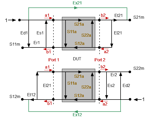
a1, a2 — incident waves, b1, b2 — reflected waves
S11a, S21a, S12a, S22a — actual value of DUT parameters
S11m, S21m, S12m, S22m — measured DUT parameters values
Two-port error model
For normalization the stimulus value is taken equal to 1. All the values used in the model are complex. The measurement result in a two-port system is affected by twelve systematic error terms.
These terms are also described in the table below.
Description |
Stimulus Source |
|
|---|---|---|
Port 1 |
Port 2 |
|
Directivity |
Ed1 |
Ed2 |
Source match |
Es1 |
Es2 |
Reflection tracking |
Er1 |
Er2 |
Transmission tracking |
Et1 |
Et2 |
Load match |
El1 |
El2 |
Isolation |
Ex1 |
Ex2 |
After determining all twelve error terms for each measurement frequency by means of a two-port calibration, it is possible to calculate the actual value of the S-parameters: S11a, S21a, S12a, S22a.
There are simplified methods, which eliminate the effect of only one or several of the twelve systematic error terms.
note |
When using a two-port calibration, all four measurements S11m, S21m, S12m, S22m need to be known to determine any S-parameters. That is why updating one or all S-parameters necessitates two sweeps: first with Port 1 as a signal source, and then with Port 2 as a signal source. |
For a detailed description of calibration methods, see Calibration Methods and Procedures.